Running a Lasso Regression Analysis for polityscore
A lasso regression analysis was conducted to identify a subset of variables from a pool of 13 quantitative predictor variables that best predicted a quantitative response variable measuring Polityscore in 213 Countries. Categorical predictors included
internetuserate
incomeperperson
urbanrate
alcconsumption
armedforcesrate
co2emissions
femaleemployrate
hivrate
lifeexpectancy
oilperperson
relectricperperson
suicideper100th
employrate
All predictor variables were standardized to have a mean of zero and a standard deviation of one.
Data were randomly split into a training set that included 70% of the observations (N=213) and a test set that included 30% of the observations (N=63). The least angle regression algorithm with k=10 fold cross validation was used to estimate the lasso regression model in the training set, and the model was validated using the test set. The change in the cross validation average (mean) squared error at each step was used to identify the best subset of predictor variables.
Figure 1 Change in the validation mean square error at each step
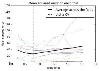
Of the 13 predictor variables, 3 were retained in the selected model. During the estimation process, internetuserate were most strongly positive associated with polityscore, and followed by armedforcesrate were most strongly negatively associated with polityscore. Other predictors associated with greater polityscore included incomeperperson,
Figure 2 Regression Coefficients Progression for Lasso Paths
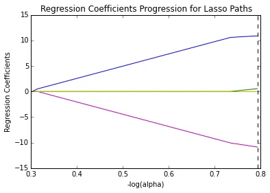
These 3 variables accounted for 40.4% of the variance in the polityscore response variable.
Code
#!/usr/bin/env python3
# vim: set fileencoding=utf-8 :
# -*- coding: utf-8 -*-
#
#       week3.py
#       Copyright 2015 arpagon
#
#       This program is free software; you can redistribute it and/or modify
#       it under the terms of the GNU General Public License as published by
#       the Free Software Foundation; either version 2 of the License, or
#       (at your option) any later version.
#
#       This program is distributed in the hope that it will be useful,
#       but WITHOUT ANY WARRANTY; without even the implied warranty of
#       MERCHANTABILITY or FITNESS FOR A PARTICULAR PURPOSE.  See the
#       GNU General Public License for more details.
#
#       You should have received a copy of the GNU General Public License
#       along with this program; if not, write to the Free Software
#       Foundation, Inc., 51 Franklin Street, Fifth Floor, Boston,
#       MA 02110-1301, USA.

"""
Running a Lasso Regression Analysis
polityscore

On dataset of gapminder
"""

__version__ = "0.0.1"
__license__ = """The GNU General Public License (GPL-2.0)"""
__author__ = "Sebastian Rojo  @arpagon"
__contributors__ = []
_debug = 0

_question="Can the Internet use democratizes society?"
_hypothesis='''
I am convinced, a deep democracy promotes the welfare of all people actively
involved in the democratic process. Some years ago while reading the book
Why Nations Fail. Suggested the deep relationship between poverty and
lawlessness in the building of democratic institutions.
'''

import pandas
import numpy as np
import matplotlib.pylab as plt
from sklearn.cross_validation import train_test_split
from sklearn.linear_model import LassoLarsCV
from sklearn import preprocessing

#%%# Data Managment 1

data = pandas.read_csv("../gapminder.csv", low_memory=False)

#Preapare Dataset
data['polityscore']=pandas.to_numeric(data['polityscore'], errors='coerce')


data['incomeperperson']=pandas.to_numeric(data['incomeperperson'], errors='coerce')
data['alcconsumption']=pandas.to_numeric(data['alcconsumption'], errors='coerce')
data['armedforcesrate']=pandas.to_numeric(data['armedforcesrate'], errors='coerce')
data['breastcancerper100th']=pandas.to_numeric(data['breastcancerper100th'], errors='coerce')
data['co2emissions']=pandas.to_numeric(data['co2emissions'], errors='coerce')
data['femaleemployrate']=pandas.to_numeric(data['femaleemployrate'], errors='coerce')
data['hivrate']=pandas.to_numeric(data['hivrate'], errors='coerce')
data['internetuserate']=pandas.to_numeric(data['internetuserate'], errors='coerce')
data['lifeexpectancy']=pandas.to_numeric(data['lifeexpectancy'], errors='coerce')
data['oilperperson']=pandas.to_numeric(data['oilperperson'], errors='coerce')
data['relectricperperson']=pandas.to_numeric(data['relectricperperson'], errors='coerce')
data['suicideper100th']=pandas.to_numeric(data['suicideper100th'], errors='coerce')
data['employrate']=pandas.to_numeric(data['employrate'], errors='coerce')
data['urbanrate']=pandas.to_numeric(data['urbanrate'], errors='coerce')

print('''
Chosee the Countrys whit a unperfect democracy as comparation point
''')

data['polityscore2']=pandas.cut(data.polityscore, [-10, 9 , 10], labels=[0,1])
data['polityscore2']=pandas.to_numeric(data['polityscore2'], errors='coerce')

data_clean = data.dropna()

data_clean.dtypes
data_clean.describe()


print('Dataset gapminder \n')

print('Obeservations:', len(data)) #number of observations (rows)
print('Variables:', len(data.columns)) # number of variables (columns)

print('\n\nTarget Variable chosen for the study are: polityscore')
print('Predictors variables for the assignment:',
                         'internetuserate','incomeperperson','urbanrate',
                         'alcconsumption', 'armedforcesrate',
                         'breastcancerper100th', 'co2emissions',
                         'femaleemployrate', 'hivrate', 'lifeexpectancy',
                         'oilperperson', 'relectricperperson',
                         'suicideper100th', 'employrate',)

#%%# Split into training and testing sets
predictors = data_clean[['internetuserate','incomeperperson','urbanrate',
                         'alcconsumption', 'armedforcesrate',
                         'co2emissions',
                         'femaleemployrate', 'hivrate', 'lifeexpectancy',
                         'oilperperson', 'relectricperperson',
                         'suicideper100th', 'employrate',
                         ]]

target = data_clean.polityscore

predictors['internetuserate']=preprocessing.scale(predictors['internetuserate'].astype('float64'))
predictors['incomeperperson']=preprocessing.scale(predictors['incomeperperson'].astype('float64'))
predictors['urbanrate']=preprocessing.scale(predictors['urbanrate'].astype('float64'))
predictors['alcconsumption']=preprocessing.scale(predictors['alcconsumption'].astype('float64'))
predictors['armedforcesrate']=preprocessing.scale(predictors['armedforcesrate'].astype('float64'))
#predictors['breastcancerper100th']=preprocessing.scale(predictors['breastcancerper100th'].astype('float64'))
predictors['co2emissions']=preprocessing.scale(predictors['co2emissions'].astype('float64'))
predictors['femaleemployrate']=preprocessing.scale(predictors['femaleemployrate'].astype('float64'))
predictors['lifeexpectancy']=preprocessing.scale(predictors['lifeexpectancy'].astype('float64'))
predictors['oilperperson']=preprocessing.scale(predictors['oilperperson'].astype('float64'))
predictors['relectricperperson']=preprocessing.scale(predictors['relectricperperson'].astype('float64'))
predictors['suicideper100th']=preprocessing.scale(predictors['suicideper100th'].astype('float64'))
predictors['employrate']=preprocessing.scale(predictors['employrate'].astype('float64'))

# split data into train and test sets
pred_train, pred_test, tar_train, tar_test = train_test_split(predictors, target,
                                                              test_size=.3, random_state=123)
print(pred_train.shape)
print(pred_test.shape)
print(tar_train.shape)
print(tar_test.shape)


#%%# specify the lasso regression model
model=LassoLarsCV(cv=10, precompute=False).fit(pred_train,tar_train)

# print variable names and regression coefficients
print('''variable names and regression coefficients''' )
print(dict(zip(predictors.columns, model.coef_)))

#%%# plot coefficient progression
m_log_alphas = -np.log10(model.alphas_)
ax = plt.gca()
plt.plot(m_log_alphas, model.coef_path_.T)
plt.axvline(-np.log10(model.alpha_), linestyle='--', color='k',
            label='alpha CV')
plt.ylabel('Regression Coefficients')
plt.xlabel('-log(alpha)')
plt.title('Regression Coefficients Progression for Lasso Paths')

#%%# plot mean square error for each fold
m_log_alphascv = -np.log10(model.cv_alphas_)
plt.figure()
plt.plot(m_log_alphascv, model.cv_mse_path_, ':')
plt.plot(m_log_alphascv, model.cv_mse_path_.mean(axis=-1), 'k',
         label='Average across the folds', linewidth=2)
plt.axvline(-np.log10(model.alpha_), linestyle='--', color='k',
            label='alpha CV')
plt.legend()
plt.xlabel('-log(alpha)')
plt.ylabel('Mean squared error')
plt.title('Mean squared error on each fold')


#%%# Calculatin R-Scaure and MRE

## MSE from training and test data
from sklearn.metrics import mean_squared_error
train_error = mean_squared_error(tar_train, model.predict(pred_train))
test_error = mean_squared_error(tar_test, model.predict(pred_test))
print ('training data MSE')
print(train_error)
print ('test data MSE')
print(test_error)

# R-square from training and test data
rsquared_train=model.score(pred_train,tar_train)
rsquared_test=model.score(pred_test,tar_test)
print ('training data R-square')
print(rsquared_train)
print ('test data R-square')
print(rsquared_test)


print(dict(zip(predictors.columns, model.coef_)))
Result
Chosee the Countrys whit a unperfect democracy as comparation point

Dataset gapminder

Obeservations: 213
Variables: 17


Target Variable chosen for the study are: polityscore
Predictors variables for the assignment: internetuserate incomeperperson urbanrate alcconsumption armedforcesrate breastcancerper100th co2emissions femaleemployrate hivrate lifeexpectancy oilperperson relectricperperson suicideper100th employrate
(38, 13)
(17, 13)
(38,)
(17,)
variable names and regression coefficients
{'co2emissions': 0.0, 'armedforcesrate': -1.571295895816798, 'lifeexpectancy': 0.0, 'employrate': 0.0, 'suicideper100th': 0.0, 'alcconsumption': 0.0, 'hivrate': 0.0, 'internetuserate': 1.7143192424041518, 'incomeperperson': 0.085369019369890664, 'urbanrate': 0.0, 'relectricperperson': 0.0, 'femaleemployrate': 0.0, 'oilperperson': 0.0}
training data MSE
21.4786054848
test data MSE
18.3721369453
training data R-square
0.404117152681
test data R-square
-0.0480749264108
{'co2emissions': 0.0, 'armedforcesrate': -1.571295895816798, 'lifeexpectancy': 0.0, 'employrate': 0.0, 'suicideper100th': 0.0, 'alcconsumption': 0.0, 'hivrate': 0.0, 'internetuserate': 1.7143192424041518, 'incomeperperson': 0.085369019369890664, 'urbanrate': 0.0, 'relectricperperson': 0.0, 'femaleemployrate': 0.0, 'oilperperson': 0.0}