Running a k-means Cluster Analysis
A k-means cluster analysis was conducted to identify underlying subgroups of Countries based on their similarity of on 11 macro-economic variables that represent characteristics that could have an impact on politycscore. Clustering variables included
‘internetuserate’, ’incomeperperson’, ’urbanrate’, ’alcconsumption’, ’armedforcesrate’, ’co2emissions’, ’lifeexpectancy’, ’oilperperson’, ’relectricperperson’, ’suicideper100th’, ’employrate’
All clustering variables were standardized to have a mean of 0 and a standard deviation of 1.
Data were randomly split into a training set that included 70% of the observations (N=40) and a test set that included 30% of the observations (N=18). A series of k-means cluster analyses were conducted on the training data specifying k=1-9 clusters, using Euclidean distance. The variance in the clustering variables that was accounted for by the clusters (r-square) was plotted for each of the nine cluster solutions in an elbow curve to provide guidance for choosing the number of clusters to interpret.
**Figure 1. Elbow curve of r-square values for the nine cluster solutions
** 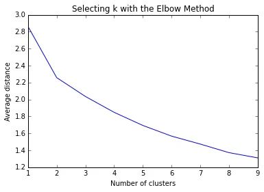
The elbow curve was inconclusive, suggesting that the 2, 3 solutions might be interpreted. The results below are for an interpretation of the 3-cluster solution.
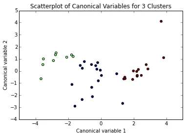
Canonical discriminant analyses was used to reduce the 11 clustering variable down a few variables that accounted for most of the variance in the clustering variables. A scatterplot of the first two canonical variables by cluster (Figure 2 shown below)
**Figure 2. Scatterplot of Canonical Variables for 3 Clusters
** 
Cluster Analysis

Cluster 0
The means on the clustering variables showed that, compared to the other clusters, Countries in cluster 1 had moderate levels on the clustering variables. They are misnamed “Developing country” on .
**Cluster 1
**
cluster 2 had higher levels on the clustering variables compared to cluster 1, Are the misnamed “Heavily indebted poor countries”
Cluster 3
cluster 3 had higher levels on the clustering variables compared to cluster 1, Are the misnamed** “Developed country”**
In order to externally validate the clusters, an Analysis of Variance (ANOVA) was conducting to test for significant differences between the clusters on politycscore. A tukey test was used for post hoc comparisons between the clusters.
Results indicated significant differences between the clusters on** **politycscore.
cluster 0 5.000000 1 0.777778 2 8.714286 standard deviations for polityscore by cluster polityscore cluster 0 6.442049 1 7.758508 2 4.810702
Code:
##

##

#!/usr/bin/env python3
# vim: set fileencoding=utf-8 :
# -*- coding: utf-8 -*-
#
#       week3.py
#       Copyright 2015 arpagon
#
#       This program is free software; you can redistribute it and/or modify
#       it under the terms of the GNU General Public License as published by
#       the Free Software Foundation; either version 2 of the License, or
#       (at your option) any later version.
#
#       This program is distributed in the hope that it will be useful,
#       but WITHOUT ANY WARRANTY; without even the implied warranty of
#       MERCHANTABILITY or FITNESS FOR A PARTICULAR PURPOSE.  See the
#       GNU General Public License for more details.
#
#       You should have received a copy of the GNU General Public License
#       along with this program; if not, write to the Free Software
#       Foundation, Inc., 51 Franklin Street, Fifth Floor, Boston,
#       MA 02110-1301, USA.

"""
Running a k-means Cluster Analysis
polityscore

On dataset of gapminder
"""

__version__ = "0.0.1"
__license__ = """The GNU General Public License (GPL-2.0)"""
__author__ = "Sebastian Rojo  @arpagon"
__contributors__ = []
_debug = 0

_question="Can the Internet use democratizes society?"
_hypothesis='''
I am convinced, a deep democracy promotes the welfare of all people actively
involved in the democratic process. Some years ago while reading the book
Why Nations Fail. Suggested the deep relationship between poverty and
lawlessness in the building of democratic institutions.
'''

import pandas
import numpy as np
import statsmodels.formula.api as smf
import statsmodels.stats.multicomp as multi
import matplotlib.pylab as plt

from pandas import Series, DataFrame
from sklearn.cross_validation import train_test_split
from sklearn import preprocessing
from sklearn.cluster import KMeans
from sklearn.decomposition import PCA

#%%# Data Managment 1

data = pandas.read_csv("../gapminder.csv", low_memory=False)

#Preapare Dataset
data['polityscore']=pandas.to_numeric(data['polityscore'], errors='coerce')

data['internetuserate']=pandas.to_numeric(data['internetuserate'], errors='coerce')
data['incomeperperson']=pandas.to_numeric(data['incomeperperson'], errors='coerce')
data['urbanrate']=pandas.to_numeric(data['urbanrate'], errors='coerce')
data['alcconsumption']=pandas.to_numeric(data['alcconsumption'], errors='coerce')
data['armedforcesrate']=pandas.to_numeric(data['armedforcesrate'], errors='coerce')
data['co2emissions']=pandas.to_numeric(data['co2emissions'], errors='coerce')
data['lifeexpectancy']=pandas.to_numeric(data['lifeexpectancy'], errors='coerce')
data['oilperperson']=pandas.to_numeric(data['oilperperson'], errors='coerce')
data['relectricperperson']=pandas.to_numeric(data['relectricperperson'], errors='coerce')
data['suicideper100th']=pandas.to_numeric(data['suicideper100th'], errors='coerce')
data['employrate']=pandas.to_numeric(data['employrate'], errors='coerce')

print('''
Chosee the Countrys whit a unperfect democracy as comparation point
''')

data['polityscore2']=pandas.cut(data.polityscore, [-10, 9 , 10], labels=[0,1])
data['polityscore2']=pandas.to_numeric(data['polityscore2'], errors='coerce')

data_clean = data.dropna()

data_clean.dtypes
data_clean.describe()

print('Dataset gapminder \n')

print('Obeservations:', len(data)) #number of observations (rows)
print('Variables:', len(data.columns)) # number of variables (columns)

print('\n\nTarget Variable chosen for the study are: polityscore')
print('Cluster variables for the assignment:',
                         'internetuserate',
                         'incomeperperson',
                         'urbanrate',
                         'alcconsumption',
                         'armedforcesrate',
                         'co2emissions',
                         'lifeexpectancy',
                         'oilperperson',
                         'relectricperperson',
                         'suicideper100th',
                         'employrate')

#%%# Split into training and testing sets
cluster = data_clean[['internetuserate',
                      'incomeperperson',
                      'urbanrate',
                      'alcconsumption',
                      'armedforcesrate',
                      'co2emissions',
                      'lifeexpectancy',
                      'oilperperson',
                      'relectricperperson',
                      'suicideper100th',
                      'employrate']]

print(cluster.describe())

clustervar=cluster.copy()

clustervar['internetuserate']=preprocessing.scale(clustervar['internetuserate'].astype('float64'))
clustervar['incomeperperson']=preprocessing.scale(clustervar['incomeperperson'].astype('float64'))
clustervar['urbanrate']=preprocessing.scale(clustervar['urbanrate'].astype('float64'))
clustervar['alcconsumption']=preprocessing.scale(clustervar['alcconsumption'].astype('float64'))
clustervar['armedforcesrate']=preprocessing.scale(clustervar['armedforcesrate'].astype('float64'))
clustervar['co2emissions']=preprocessing.scale(clustervar['co2emissions'].astype('float64'))
clustervar['lifeexpectancy']=preprocessing.scale(clustervar['lifeexpectancy'].astype('float64'))
clustervar['oilperperson']=preprocessing.scale(clustervar['oilperperson'].astype('float64'))
clustervar['relectricperperson']=preprocessing.scale(clustervar['relectricperperson'].astype('float64'))
clustervar['suicideper100th']=preprocessing.scale(clustervar['suicideper100th'].astype('float64'))
clustervar['employrate']=preprocessing.scale(clustervar['employrate'].astype('float64'))

# split data into train and test sets
clus_train, clus_test = train_test_split(clustervar, test_size=.3,
                                                              random_state=123)

print(clus_train.shape)
print(clus_test.shape)

#%%# k-means cluster analysis for 1-9 clusters
from scipy.spatial.distance import cdist
clusters=range(1,10)
meandist=[]

for k in clusters:
    model=KMeans(n_clusters=k)
    model.fit(clus_train)
    clusassign=model.predict(clus_train)
    meandist.append(sum(np.min(cdist(clus_train, model.cluster_centers_, 'euclidean'), axis=1))
    / clus_train.shape[0])

#%%# Plot average distance from observations from the cluster centroid
"""
Plot average distance from observations from the cluster centroid
to use the Elbow Method to identify number of clusters to choose
"""
plt.plot(clusters, meandist)
plt.xlabel('Number of clusters')
plt.ylabel('Average distance')
plt.title('Selecting k with the Elbow Method')
plt.show()
plt.close()

#%%# Interpret 3 cluster solution
model3=KMeans(n_clusters=3)
model3.fit(clus_train)
clusassign=model3.predict(clus_train)

#%%# plot clusters

pca_2 = PCA(2)
plot_columns = pca_2.fit_transform(clus_train)
plt.scatter(x=plot_columns[:,0], y=plot_columns[:,1], c=model3.labels_,)
plt.xlabel('Canonical variable 1')
plt.ylabel('Canonical variable 2')
plt.title('Scatterplot of Canonical Variables for 3 Clusters')
plt.show()
plt.close()

#%%# merge cluster assignment
'''
multiple steps to merge cluster assignment with clustering variables to examine
cluster variable means by cluster
'''
# create a unique identifier variable from the index for the
# cluster training data to merge with the cluster assignment variable
clus_train.reset_index(level=0, inplace=True)
# create a list that has the new index variable
cluslist=list(clus_train['index'])
# create a list of cluster assignments
labels=list(model3.labels_)
# combine index variable list with cluster assignment list into a dictionary
newlist=dict(zip(cluslist, labels))
print("Combined index variable list with cluster assignment")
print(newlist)

# convert newlist dictionary to a dataframe
newclus=DataFrame.from_dict(newlist, orient='index')
print("New Cluster")
print(newclus)

# rename the cluster assignment column
newclus.columns = ['cluster']

# now do the same for the cluster assignment variable
# create a unique identifier variable from the index for the
# cluster assignment dataframe
# to merge with cluster training data
newclus.reset_index(level=0, inplace=True)
# merge the cluster assignment dataframe with the cluster training variable dataframe
# by the index variable
merged_train=pandas.merge(clus_train, newclus, on='index')
merged_train.head(n=100)
# cluster frequencies
merged_train.cluster.value_counts()

#%%# calculate clustering variable means by cluster
clustergrp = merged_train.groupby('cluster').mean()
print ("Clustering variable means by cluster")
print(clustergrp)

# validate clusters in training data by examining cluster differences in polityscore using Gapinder
# first have to merge polityscore with clustering variables and cluster assignment data
polityscore_data=data_clean['polityscore']
# split polityscore data into train and test sets
polityscore_train, polityscore_test = train_test_split(polityscore_data, test_size=.3, random_state=123)
polityscore_train1=pandas.DataFrame(polityscore_train)
polityscore_train1.reset_index(level=0, inplace=True)
merged_train_all=pandas.merge(polityscore_train1, merged_train, on='index')
sub1 = merged_train_all[['polityscore', 'cluster']].dropna()

polityscoremod = smf.ols(formula='polityscore ~ C(cluster)', data=sub1).fit()
print (polityscoremod.summary())

print ('means for polityscore by cluster')
m1= sub1.groupby('cluster').mean()
print (m1)

print ('standard deviations for polityscore by cluster')
m2= sub1.groupby('cluster').std()
print (m2)

mc1 = multi.MultiComparison(sub1['polityscore'], sub1['cluster'])
res1 = mc1.tukeyhsd()
print(res1.summary())
Result:
Python 3.4.3+ (default, Oct 14 2015, 16:03:50)
Type "copyright", "credits" or "license" for more information.

IPython 2.3.0 -- An enhanced Interactive Python.
?         -> Introduction and overview of IPython's features.
%quickref -> Quick reference.
help      -> Python's own help system.
object?   -> Details about 'object', use 'object??' for extra details.
%guiref   -> A brief reference about the graphical user interface.

In [1]: runfile('/home/arpagon/Workspace/DataAnalysisSpecialization/src/Machine Learning/week4.py', wdir='/home/arpagon/Workspace/DataAnalysisSpecialization/src/Machine Learning')

Chosee the Countrys whit a unperfect democracy as comparation point

Dataset gapminder

Obeservations: 213
Variables: 17

Target Variable chosen for the study are: polityscore
Cluster variables for the assignment: internetuserate incomeperperson urbanrate alcconsumption armedforcesrate co2emissions lifeexpectancy oilperperson relectricperperson suicideper100th employrate
       internetuserate  incomeperperson   urbanrate  alcconsumption  count        58.000000        58.000000   58.000000       58.000000
mean         51.249216     12444.391557   67.865862        9.307931
std          26.598757     12335.594804   16.466697        5.232932
min           2.199998       558.062877   27.140000        0.050000
25%          32.384640      2498.678807   60.805000        6.192500
50%          46.333146      5869.642345   68.570000        9.870000
75%          77.097878     24657.106188   77.780000       12.945000
max          93.277508     39972.352768  100.000000       19.150000

       armedforcesrate  co2emissions  lifeexpectancy  oilperperson  count        58.000000  5.800000e+01       58.000000     58.000000
mean          1.260754  1.631592e+10       75.265862      1.275188
std           1.057948  4.610825e+10        5.839142      1.682150
min           0.287892  2.262553e+08       52.797000      0.032281
25%           0.534841  1.890118e+09       73.013250      0.461774
50%           0.943844  3.852409e+09       75.539000      0.867870
75%           1.641310  1.053362e+10       80.521250      1.562843
max           6.394936  3.342209e+11       83.394000     12.228645

       relectricperperson  suicideper100th  employrate
count           58.000000        58.000000   58.000000
mean          1543.790545        10.956465   57.536207
std           1887.521465         6.948989    7.398879
min             68.115229         1.380965   41.099998
25%            487.615567         5.920024   52.650000
50%            875.419623         9.993177   58.450001
75%           1858.100384        13.537748   62.099999
max          11154.755033        33.341860   75.199997
(40, 11)
(18, 11)
/home/arpagon/.local/lib/python3.4/site-packages/sklearn/preprocessing/data.py:167: UserWarning: Numerical issues were encountered when centering the data and might not be solved. Dataset may contain too large values. You may need to prescale your features.
  warnings.warn("Numerical issues were encountered "


/usr/lib/python3/dist-packages/matplotlib/collections.py:571: FutureWarning: elementwise comparison failed; returning scalar instead, but in the future will perform elementwise comparison
  if self._edgecolors == str('face'):


Combined index variable list with cluster assignment
{96: 0, 139: 2, 197: 1, 6: 0, 72: 0, 201: 2, 202: 2, 11: 0, 205: 1, 207: 0, 144: 2, 152: 1, 146: 1, 84: 0, 86: 1, 25: 0, 88: 1, 153: 0, 154: 0, 90: 2, 69: 2, 159: 0, 32: 2, 16: 0, 100: 0, 9: 2, 39: 0, 178: 1, 174: 0, 136: 2, 50: 2, 179: 0, 54: 0, 55: 1, 184: 2, 185: 2, 124: 0, 10: 2, 190: 1, 63: 2}
New Cluster
     0
96   0
139  2
197  1
6    0
72   0
201  2
202  2
11   0
205  1
207  0
144  2
152  1
146  1
84   0
86   1
25   0
88   1
153  0
154  0
90   2
69   2
159  0
32   2
16   0
100  0
9    2
39   0
178  1
174  0
136  2
50   2
179  0
54   0
55   1
184  2
185  2
124  0
10   2
190  1
63   2
Clustering variable means by cluster
              index  internetuserate  incomeperperson  urbanrate  cluster
0         97.235294        -0.122710        -0.438748   0.198336
1        144.111111        -1.335951        -0.868176  -1.289793
2        108.142857         1.198233         1.251260   0.625008

         alcconsumption  armedforcesrate  co2emissions  lifeexpectancy  cluster
0              0.596728         0.225199     -0.205747       -0.051477
1             -1.022763        -0.037247     -0.190892       -1.369818
2              0.240118        -0.541950     -0.067069        0.898356

         oilperperson  relectricperperson  suicideper100th  employrate
cluster
0           -0.214412           -0.359952         0.114257   -0.077916
1           -0.463567           -0.602981        -0.232547   -0.471509
2            0.450235            1.121878        -0.145282    0.594942
                            OLS Regression Results
==============================================================================
Dep. Variable:            polityscore   R-squared:                       0.194
Model:                            OLS   Adj. R-squared:                  0.151
Method:                 Least Squares   F-statistic:                     4.460
Date:                Thu, 05 May 2016   Prob (F-statistic):             0.0184
Time:                        14:48:28   Log-Likelihood:                -128.52
No. Observations:                  40   AIC:                             263.0
Df Residuals:                      37   BIC:                             268.1
Df Model:                           2
Covariance Type:            nonrobust
===================================================================================
                      coef    std err          t      P>|t|      [95.0% Conf. Int.]
-----------------------------------------------------------------------------------
Intercept           5.0000      1.516      3.297      0.002         1.927     8.073
C(cluster)[T.1]    -4.2222      2.577     -1.638      0.110        -9.445     1.000
C(cluster)[T.2]     3.7143      2.257      1.646      0.108        -0.858     8.286
==============================================================================
Omnibus:                        9.265   Durbin-Watson:                   2.187
Prob(Omnibus):                  0.010   Jarque-Bera (JB):                8.831
Skew:                          -1.135   Prob(JB):                       0.0121
Kurtosis:                       3.381   Cond. No.                         3.45
==============================================================================

Warnings:
[1] Standard Errors assume that the covariance matrix of the errors is correctly specified.
means for polityscore by cluster
         polityscore
cluster
0           5.000000
1           0.777778
2           8.714286
standard deviations for polityscore by cluster
         polityscore
cluster
0           6.442049
1           7.758508
2           4.810702
Multiple Comparison of Means - Tukey HSD,FWER=0.05
==============================================
group1 group2 meandiff  lower    upper  reject
----------------------------------------------
  0      1    -4.2222  -10.5143  2.0698 False
  0      2     3.7143  -1.7944   9.2229 False
  1      2     7.9365   1.4153  14.4578  True
----------------------------------------------

In [2]: