Can the Internet use democratizes society? Test a Multiple Regression Model
Question: Can the Internet use democratizes society?
hypothesis: I am convinced, a deep democracy promotes the welfare of all people actively involved in the democratic process. Some years ago while reading the book Why Nations Fail. Suggested the deep relationship between poverty and lawlessness in the building of democratic institutions.
Code:
#!/usr/bin/env python
# vim: set fileencoding=utf-8 :
# -*- coding: utf-8 -*-
#
#       week3.py
#       Copyright 2015 arpagon
#
#       This program is free software; you can redistribute it and/or modify
#       it under the terms of the GNU General Public License as published by
#       the Free Software Foundation; either version 2 of the License, or
#       (at your option) any later version.
#
#       This program is distributed in the hope that it will be useful,
#       but WITHOUT ANY WARRANTY; without even the implied warranty of
#       MERCHANTABILITY or FITNESS FOR A PARTICULAR PURPOSE.  See the
#       GNU General Public License for more details.
#
#       You should have received a copy of the GNU General Public License
#       along with this program; if not, write to the Free Software
#       Foundation, Inc., 51 Franklin Street, Fifth Floor, Boston,
#       MA 02110-1301, USA.

"""
Test a Basic Linear Regression Model
polityscore, internetuserate, incomeperperson.

On dataset of gapminder
"""

__version__ = "0.0.1"
__license__ = """The GNU General Public License (GPL-2.0)"""
__author__ = "Sebastian Rojo  @arpagon"
__contributors__ = []
_debug = 0

_question="Can the Internet use democratizes society?"
_hypothesis='''
I am convinced, a deep democracy promotes the welfare of all people actively
involved in the democratic process. Some years ago while reading the book
Why Nations Fail. Suggested the deep relationship between poverty and
lawlessness in the building of democratic institutions.
'''

import pandas
import numpy
import seaborn as sns
import scipy
import matplotlib.pyplot as plt
import statsmodels.api as sm
import statsmodels.formula.api as smf


data = pandas.read_csv("../gapminder.csv", low_memory=False)

print('Dataset gapminder \n')

print('Obeservations:', len(data)) #number of observations (rows)
print('Variables:', len(data.columns)) # number of variables (columns)

print('\n\nVariables chosen for the study are: internetuserate, polityscore')
print('Additional variables for the assignment: urbanrate, incomeperperson')

#Preapare Dataset
data['internetuserate'] = data['internetuserate'].convert_objects(
                                                        convert_numeric=True)
data['polityscore'] = data['polityscore'].convert_objects(
                                                        convert_numeric=True)
data['incomeperperson'] = data['incomeperperson'].convert_objects(
                                                        convert_numeric=True)
data['urbanrate'] = data['urbanrate'].convert_objects(
                                                        convert_numeric=True)


data['internetuserate']=data['internetuserate'].replace(' ', numpy.nan)
data['polityscore']=data['polityscore'].replace(' ', numpy.nan)
data['incomeperperson']=data['incomeperperson'].replace(' ', numpy.nan)
data['urbanrate']=data['urbanrate'].replace(' ', numpy.nan)


sub1=data[['country',
           'internetuserate',
            'polityscore',
            'incomeperperson',
            'urbanrate']].dropna()

#%%#  POLYNOMIAL REGRESSION


#basic scatterplot:  Q->Q
plt.figure()
scat1 = sns.regplot(x="internetuserate", y="polityscore", data=sub1)
plt.xlabel('Internet Use Rate')
plt.ylabel('Overall polity score')
plt.title('Scatterplot for the Association Between Internet Use Rate and' \
                                                        'Overall polity score')
plt.show()
plt.close()

# fit second order polynomial
# run the 2 scatterplots together to get both linear and second order fit lines

plt.figure()
scat1 = sns.regplot(x="internetuserate", y="polityscore", order=2, data=sub1)
plt.xlabel('Internet Use Rate')
plt.ylabel('Overall polity score')
plt.title('Scatterplot for the Association Between Internet Use Rate and' \
                                                        'Overall polity score')
plt.show()
plt.close()

# center quantitative IVs for regression analysis
sub1['internetuserate_c'] = (sub1['internetuserate'] - sub1['internetuserate'].mean())
sub1['incomeperperson_c'] = (sub1['incomeperperson'] - sub1['incomeperperson'].mean())
sub1['urbanrate_c'] = (sub1['urbanrate'] - sub1['urbanrate'].mean())
print(sub1[["internetuserate_c","incomeperperson_c", "urbanrate_c"]].describe())

# linear regression analysis
reg1 = smf.ols('polityscore ~ internetuserate_c', data=sub1).fit()
print (reg1.summary())
# quadratic (polynomial) regression analysis

reg2 = smf.ols('polityscore ~ internetuserate_c + I(internetuserate_c**2)', data=sub1).fit()
print (reg2.summary())


#%%# EVALUATING MODEL FIT

print("Dicard Cuadratic internetuserate_c not fit in Model")

# adding internet use rate
reg3 = smf.ols('polityscore  ~  internetuserate_c + urbanrate_c + incomeperperson_c',
               data=sub1).fit()
print (reg3.summary())


#Q-Q plot for normality
fig4=sm.qqplot(reg3.resid, line='r')


# simple plot of residuals
plt.figure()
stdres=pandas.DataFrame(reg3.resid_pearson)
plt.plot(stdres, 'o', ls='None')
l = plt.axhline(y=0, color='r')
plt.ylabel('Standardized Residual')
plt.xlabel('Observation Number')
plt.show()
plt.close()


# additional regression diagnostic plots
plt.figure()
fig2 = plt.figure(figsize=(12,8))
fig2 = sm.graphics.plot_regress_exog(reg3,  "urbanrate_c", fig=fig2)
plt.show()
plt.close()


# leverage plot
fig3=sm.graphics.influence_plot(reg3, size=8)
print(fig3)
Results:
runfile('/home/arpagon/Workspace/DataAnalysisSpecialization/src/Regression Modeling in Practice/week3.py', wdir='/home/arpagon/Workspace/DataAnalysisSpecialization/src/Regression Modeling in Practice')
Dataset gapminder

Obeservations: 213
Variables: 16


Variables chosen for the study are: internetuserate, polityscore
Additional variables for the assignment: urbanrate, incomeperperson


       internetuserate_c  incomeperperson_c   urbanrate_c
count       1.530000e+02       1.530000e+02  1.530000e+02
mean       -2.461357e-15       3.299147e-12  9.845429e-15
std         2.755326e+01       9.792742e+03  2.249083e+01
min        -3.247217e+01      -6.581954e+03 -4.489739e+01
25%        -2.431203e+01      -6.089856e+03 -1.847739e+01
50%        -5.942212e+00      -4.463395e+03  1.982614e+00
75%         1.923195e+01       6.088228e+01  1.632261e+01
max         6.059527e+01       3.328662e+04  4.470261e+01
                            OLS Regression Results
==============================================================================
Dep. Variable:            polityscore   R-squared:                       0.135
Model:                            OLS   Adj. R-squared:                  0.130
Method:                 Least Squares   F-statistic:                     23.64
Date:                Mon, 25 Jan 2016   Prob (F-statistic):           2.88e-06
Time:                        23:16:00   Log-Likelihood:                -484.91
No. Observations:                 153   AIC:                             973.8
Df Residuals:                     151   BIC:                             979.9
Df Model:                           1
Covariance Type:            nonrobust
=====================================================================================
                        coef    std err          t      P>|t|      [95.0% Conf. Int.]
-------------------------------------------------------------------------------------
Intercept             3.9412      0.468      8.413      0.000         3.016     4.867
internetuserate_c     0.0829      0.017      4.862      0.000         0.049     0.117
==============================================================================
Omnibus:                       23.318   Durbin-Watson:                   2.010
Prob(Omnibus):                  0.000   Jarque-Bera (JB):               29.690
Skew:                          -1.075   Prob(JB):                     3.57e-07
Kurtosis:                       3.193   Cond. No.                         27.5
==============================================================================

Warnings:
[1] Standard Errors assume that the covariance matrix of the errors is correctly specified.
                            OLS Regression Results
==============================================================================
Dep. Variable:            polityscore   R-squared:                       0.136
Model:                            OLS   Adj. R-squared:                  0.124
Method:                 Least Squares   F-statistic:                     11.81
Date:                Mon, 25 Jan 2016   Prob (F-statistic):           1.73e-05
Time:                        23:16:00   Log-Likelihood:                -484.85
No. Observations:                 153   AIC:                             975.7
Df Residuals:                     150   BIC:                             984.8
Df Model:                           2
Covariance Type:            nonrobust
=============================================================================================
                                coef    std err          t      P>|t|      [95.0% Conf. Int.]
---------------------------------------------------------------------------------------------
Intercept                     3.7579      0.726      5.177      0.000         2.324     5.192
internetuserate_c             0.0789      0.021      3.770      0.000         0.038     0.120
I(internetuserate_c ** 2)     0.0002      0.001      0.331      0.741        -0.001     0.002
==============================================================================
Omnibus:                       22.801   Durbin-Watson:                   2.015
Prob(Omnibus):                  0.000   Jarque-Bera (JB):               28.856
Skew:                          -1.060   Prob(JB):                     5.42e-07
Kurtosis:                       3.178   Cond. No.                     1.68e+03
==============================================================================

Warnings:
[1] Standard Errors assume that the covariance matrix of the errors is correctly specified.
[2] The condition number is large, 1.68e+03. This might indicate that there are
strong multicollinearity or other numerical problems.
Dicard Cuadratic internetuserate_c not fit in Model
                            OLS Regression Results
==============================================================================
Dep. Variable:            polityscore   R-squared:                       0.144
Model:                            OLS   Adj. R-squared:                  0.127
Method:                 Least Squares   F-statistic:                     8.373
Date:                Mon, 25 Jan 2016   Prob (F-statistic):           3.51e-05
Time:                        23:16:00   Log-Likelihood:                -484.12
No. Observations:                 153   AIC:                             976.2
Df Residuals:                     149   BIC:                             988.4
Df Model:                           3
Covariance Type:            nonrobust
=====================================================================================
                        coef    std err          t      P>|t|      [95.0% Conf. Int.]
-------------------------------------------------------------------------------------
Intercept             3.9412      0.469      8.400      0.000         3.014     4.868
internetuserate_c     0.1078      0.032      3.368      0.001         0.045     0.171
urbanrate_c          -0.0336      0.028     -1.186      0.237        -0.090     0.022
incomeperperson_c -2.223e-05   8.19e-05     -0.271      0.786        -0.000     0.000
==============================================================================
Omnibus:                       21.852   Durbin-Watson:                   1.975
Prob(Omnibus):                  0.000   Jarque-Bera (JB):               27.386
Skew:                          -1.034   Prob(JB):                     1.13e-06
Kurtosis:                       3.137   Cond. No.                     9.76e+03
==============================================================================

Warnings:
[1] Standard Errors assume that the covariance matrix of the errors is correctly specified.
[2] The condition number is large, 9.76e+03. This might indicate that there are
strong multicollinearity or other numerical problems.


Figure(640x440)

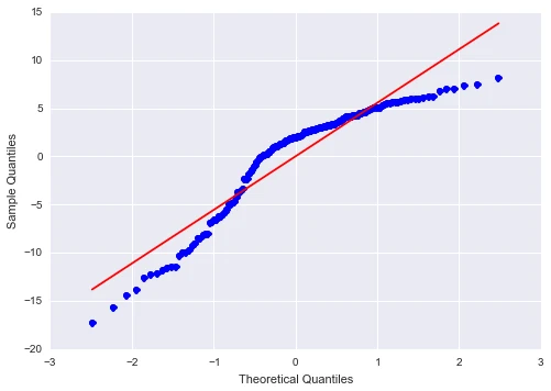
a) q-q plot
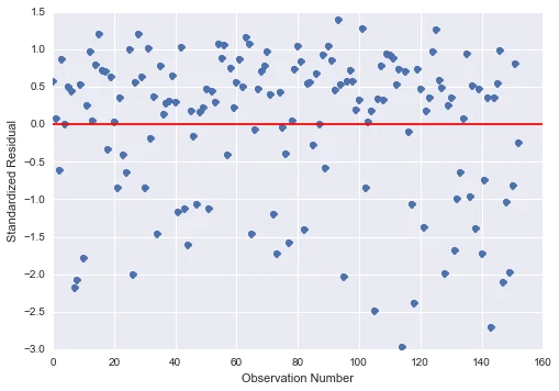
b) standardized residuals for all observations
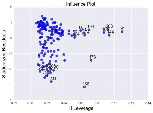
c) leverage plot
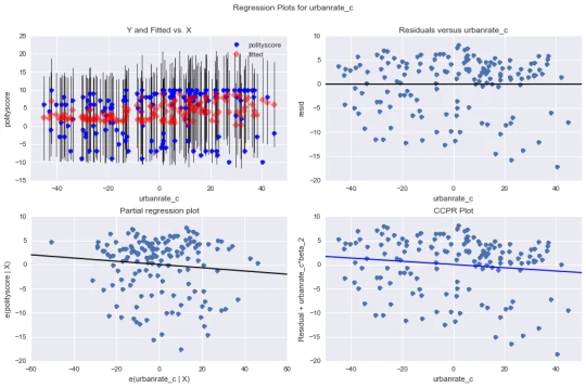
additional regression diagnostic plots
Analisys
- After adjusting for potential confounding factors, Politic Score (Beta=0.136, p=.0001) was significantly and positively associated with Internet Use Rate. When adding additional variables like urbanrate_c and incomeperperson_c ** increase the percentage of predicted values (Beta=0.144, p=.001)**
- Whatever this mean a weak relation between Politic Score and Internet Use Rate. When adding possible cofunding variables this variables get no acceptables P values.
- Adding additional variable like urbanrate_c and incomeperperson_c This variavbles is not significantly associated with Politic Score.
OLS Analysis.
                            OLS Regression Results
==============================================================================
Dep. Variable:            polityscore   R-squared:                       0.144
Model:                            OLS   Adj. R-squared:                  0.127
Method:                 Least Squares   F-statistic:                     8.373
Date:                Mon, 25 Jan 2016   Prob (F-statistic):           3.51e-05
Time:                        23:16:00   Log-Likelihood:                -484.12
No. Observations:                 153   AIC:                             976.2
Df Residuals:                     149   BIC:                             988.4
Df Model:                           3
Covariance Type:            nonrobust
=====================================================================================
                        coef    std err          t      P>|t|      [95.0% Conf. Int.]
-------------------------------------------------------------------------------------
Intercept             3.9412      0.469      8.400      0.000         3.014     4.868
internetuserate_c     0.1078      0.032      3.368      0.001         0.045     0.171
urbanrate_c          -0.0336      0.028     -1.186      0.237        -0.090     0.022
incomeperperson_c -2.223e-05   8.19e-05     -0.271      0.786        -0.000     0.000
==============================================================================
Omnibus:                       21.852   Durbin-Watson:                   1.975
Prob(Omnibus):                  0.000   Jarque-Bera (JB):               27.386
Skew:                          -1.034   Prob(JB):                     1.13e-06
Kurtosis:                       3.137   Cond. No.                     9.76e+03
==============================================================================