Can the Internet use democratizes society? Chi-Square Test of Independence
Question: Can the Internet use democratizes society?
hypothesis: I am convinced, a deep democracy promotes the welfare of all people actively involved in the democratic process. Some years ago while reading the book Why Nations Fail. Suggested the deep relationship between poverty and lawlessness in the building of democratic institutions.
Code:
#!/usr/bin/env python
# vim: set fileencoding=utf-8 :
# -*- coding: utf-8 -*-
#
#       week2.py
#       Copyright 2015 arpagon
#
#       This program is free software; you can redistribute it and/or modify
#       it under the terms of the GNU General Public License as published by
#       the Free Software Foundation; either version 2 of the License, or
#       (at your option) any later version.
#
#       This program is distributed in the hope that it will be useful,
#       but WITHOUT ANY WARRANTY; without even the implied warranty of
#       MERCHANTABILITY or FITNESS FOR A PARTICULAR PURPOSE.  See the
#       GNU General Public License for more details.
#
#       You should have received a copy of the GNU General Public License
#       along with this program; if not, write to the Free Software
#       Foundation, Inc., 51 Franklin Street, Fifth Floor, Boston,
#       MA 02110-1301, USA.

"""
Perform  analysis of variance for variables internetuserate, polityscore
urbanrate, incomeperperson.

On dataset of gapminder
"""

__version__ = "0.0.1"
__license__ = """The GNU General Public License (GPL-2.0)"""
__author__ = "Sebastian Rojo  @arpagon"
__contributors__ = []
_debug = 0

_question="Can the Internet use democratizes society?"
_hypothesis='''
I am convinced, a deep democracy promotes the welfare of all people actively
involved in the democratic process. Some years ago while reading the book
Why Nations Fail. Suggested the deep relationship between poverty and
lawlessness in the building of democratic institutions.
'''


import pandas
import numpy
import seaborn
import statsmodels.formula.api as smf
import statsmodels.stats.multicomp as multi
import matplotlib.pyplot as plt
import scipy

data = pandas.read_csv("../gapminder.csv", low_memory=False)

print('Dataset gapminder \n')

print('Obeservations:', len(data)) #number of observations (rows)
print('Variables:', len(data.columns)) # number of variables (columns)

print('\n\nVariables chosen for the study are: internetuserate, polityscore')
print('Additional variables for the assignment: urbanrate, incomeperperson')

#internetuserate
data['internetuserate'] = data['internetuserate'].convert_objects(
                                                        convert_numeric=True)
data['polityscore'] = data['polityscore'].convert_objects(
                                                        convert_numeric=True)

sub1=data[['country','internetuserate', 'polityscore']].dropna()

data_variance = sub1.copy()

print('=  categorizing explanatory variable intusegroup =')

print('intusegroup4 - 4 categories - 0 low use, 10 is massive use')
data_variance['intusegroup4']=pandas.cut(data_variance.internetuserate,
[0, 25 , 50, 75, 100],labels=[25,50,75,100])

intusegroup4_count = data_variance['intusegroup4'].value_counts(sort=False)
print (intusegroup4_count)

print('\n==Percentages for internetuserate grouped as intusegroup4 ==')
print('''Internet users (per 100 people) Internet users are people with access
to the worldwide network.''')

intusegroup4_percent = data_variance['intusegroup4'].value_counts(sort=False,
                                                                normalize=True)
print (intusegroup4_percent)

print('=  categorizing response variable polityscore =')


print('polityscore2 - 2 polityscore')
data_variance['polityscore2']=pandas.cut(data_variance.polityscore,
                                               [-10, 7 , 10], labels=[0,1])

polityscore2_count = data_variance['polityscore2'].value_counts(sort=False)
print (polityscore2_count)


print('\n==Percentages for Poltiyscore grouped as poltiyscore2 ==')
print('''Overall polity score from the Polity IV dataset, calculated by
subtracting an autocracy score from a democracy score. The summary
measure of a country's democratic and free nature. -10 is the lowest
value, 10 the highest.''')

polityscore2_percent = data_variance['polityscore2'].value_counts(sort=False,
                                                                normalize=True)
print (polityscore2_percent)

print('\n=  contingency table of observed counts =')

# contingency table of observed counts
ct1=pandas.crosstab(data_variance['polityscore2'], data_variance['intusegroup4'])
print (ct1)

print('\n=  column percentages =')

# column percentages
colsum=ct1.sum(axis=0)
colpct=ct1/colsum
print(colpct)

print ('chi-square value, p value, expected counts')
cs1= scipy.stats.chi2_contingency(ct1)
print (cs1)


# set variable types
data_variance["intusegroup4"] = data_variance["intusegroup4"].astype('category')
# new code for setting variables to numeric:

data_variance['polityscore2'] = data_variance['polityscore2'].convert_objects(
                                                        convert_numeric=True)


seaborn.factorplot(x="intusegroup4", y="polityscore2", data=data_variance, kind="bar", ci=None)
plt.ylabel('Politic Score 1:Democratic 0:inperfect democracy')
plt.show()
plt.close()

print('\n= Comparative 25 and 50 =')

recode2 = {25: 25, 50: 50}
data_variance['COMP25v50']= data_variance['intusegroup4'].map(recode2)

# contingency table of observed counts
ct2=pandas.crosstab(data_variance['polityscore2'], data_variance['COMP25v50'])
print (ct2)

# column percentages
colsum=ct2.sum(axis=0)
colpct=ct2/colsum
print(colpct)

print ('chi-square value, p value, expected counts')
cs2= scipy.stats.chi2_contingency(ct2)
print (cs2)

print('\n= Comparative 25 and 75 =')

recode3 = {25: 25, 75: 75}
data_variance['COMP25v75']= data_variance['intusegroup4'].map(recode3)

# contingency table of observed counts
ct3=pandas.crosstab(data_variance['polityscore2'], data_variance['COMP25v75'])
print (ct3)

# column percentages
colsum=ct3.sum(axis=0)
colpct=ct3/colsum
print(colpct)

print ('chi-square value, p value, expected counts')
cs3= scipy.stats.chi2_contingency(ct3)
print (cs3)

print('\n= Comparative 25 and 100 =')

recode4 = {25: 25, 100: 100}
data_variance['COMP25v100']= data_variance['intusegroup4'].map(recode4)

# contingency table of observed counts
ct4=pandas.crosstab(data_variance['polityscore2'], data_variance['COMP25v100'])
print (ct4)

# column percentages
colsum=ct4.sum(axis=0)
colpct=ct4/colsum
print(colpct)

print ('chi-square value, p value, expected counts')
cs4= scipy.stats.chi2_contingency(ct4)
print (cs4)

print('\n= Comparative 50 and  75=')

recode5 = {50: 50, 75: 75}
data_variance['COMP50v75']= data_variance['intusegroup4'].map(recode5)

# contingency table of observed counts
ct5=pandas.crosstab(data_variance['polityscore2'], data_variance['COMP50v75'])
print (ct5)

# column percentages
colsum=ct5.sum(axis=0)
colpct=ct5/colsum
print(colpct)

print ('chi-square value, p value, expected counts')
cs5= scipy.stats.chi2_contingency(ct5)
print (cs5)

print('\n= Comparative 50 and  100 =')

recode6 = {50: 50, 100: 100}
data_variance['COMP50v100']= data_variance['intusegroup4'].map(recode6)

# contingency table of observed counts
ct6=pandas.crosstab(data_variance['polityscore2'], data_variance['COMP50v100'])
print (ct6)

# column percentages
colsum=ct6.sum(axis=0)
colpct=ct6/colsum
print(colpct)

print ('chi-square value, p value, expected counts')
cs6= scipy.stats.chi2_contingency(ct6)
print (cs6)

print('\n= Comparative 75 and  100 =')

recode7 = {75: 75, 100: 100}
data_variance['COMP75v100']= data_variance['intusegroup4'].map(recode7)

# contingency table of observed counts
ct7=pandas.crosstab(data_variance['polityscore2'], data_variance['COMP75v100'])
print (ct7)

# column percentages
colsum=ct7.sum(axis=0)
colpct=ct7/colsum
print(colpct)

print ('chi-square value, p value, expected counts')
cs7= scipy.stats.chi2_contingency(ct7)
print (cs7)
Result:
runfile('/home/arpagon/Workspace/DataAnalysisSpecialization/src/Data Analysis Tools/week2.py', wdir='/home/arpagon/Workspace/DataAnalysisSpecialization/src/Data Analysis Tools')
Dataset gapminder

Obeservations: 213
Variables: 16


Variables chosen for the study are: internetuserate, polityscore
Additional variables for the assignment: urbanrate, incomeperperson
=  categorizing explanatory variable intusegroup =
intusegroup4 - 4 categories - 0 low use, 10 is massive use
25     74
50     41
75     23
100    17
dtype: int64

==Percentages for internetuserate grouped as intusegroup4 ==
Internet users (per 100 people) Internet users are people with access
to the worldwide network.
25     0.477419
50     0.264516
75     0.148387
100    0.109677
dtype: float64
=  categorizing response variable polityscore =
polityscore2 - 2 polityscore
0    87
1    66
dtype: int64

==Percentages for Poltiyscore grouped as poltiyscore2 ==
Overall polity score from the Polity IV dataset, calculated by
subtracting an autocracy score from a democracy score. The summary
measure of a country's democratic and free nature. -10 is the lowest
value, 10 the highest.
0    0.561290
1    0.425806
dtype: float64

=  contingency table of observed counts =
intusegroup4  25   50   75   100
polityscore2
0              60   22    4    1
1              14   18   19   15

=  column percentages =
intusegroup4       25    50        75      100
polityscore2
0             0.810811  0.55  0.173913  0.0625
1             0.189189  0.45  0.826087  0.9375
chi-square value, p value, expected counts
(49.069261660631597, 1.2609118937138063e-10, 3, array([[ 42.07843137,  22.74509804,  13.07843137,   9.09803922],
       [ 31.92156863,  17.25490196,   9.92156863,   6.90196078]]))


= Comparative 25 and 50 =
COMP25v50     25  50
polityscore2
0             60  22
1             14  18
COMP25v50           25    50
polityscore2
0             0.810811  0.55
1             0.189189  0.45
chi-square value, p value, expected counts
(7.5034569153757431, 0.0061580678540386433, 1, array([[ 53.22807018,  28.77192982],
       [ 20.77192982,  11.22807018]]))

= Comparative 25 and 75 =
COMP25v75     25  75
polityscore2
0             60   4
1             14  19
COMP25v75           25        75
polityscore2
0             0.810811  0.173913
1             0.189189  0.826087
chi-square value, p value, expected counts
(28.934665837094506, 7.4861091265323711e-08, 1, array([[ 48.82474227,  15.17525773],
       [ 25.17525773,   7.82474227]]))

= Comparative 25 and 100 =
COMP25v100    25   100
polityscore2
0              60    1
1              14   15
COMP25v100         25      100
polityscore2
0             0.810811  0.0625
1             0.189189  0.9375
chi-square value, p value, expected counts
(30.391698050509525, 3.5303583572118305e-08, 1, array([[ 50.15555556,  10.84444444],
       [ 23.84444444,   5.15555556]]))

= Comparative 50 and  75=
COMP50v75     50  75
polityscore2
0             22   4
1             18  19
COMP50v75       50        75
polityscore2
0             0.55  0.173913
1             0.45  0.826087
chi-square value, p value, expected counts
(7.0407504180601999, 0.0079675641424967122, 1, array([[ 16.50793651,   9.49206349],
       [ 23.49206349,  13.50793651]]))

= Comparative 50 and  100 =
COMP50v100    50   100
polityscore2
0              22    1
1              18   15
COMP50v100     50      100
polityscore2
0             0.55  0.0625
1             0.45  0.9375
chi-square value, p value, expected counts
(9.2982872200263511, 0.0022936819980624518, 1, array([[ 16.42857143,   6.57142857],
       [ 23.57142857,   9.42857143]]))

= Comparative 75 and  100 =
COMP75v100    75   100
polityscore2
0               4    1
1              19   15
COMP75v100         75      100
polityscore2
0             0.173913  0.0625
1             0.826087  0.9375
chi-square value, p value, expected counts
(0.28816735933503818, 0.59139732995039396, 1, array([[  2.94871795,   2.05128205],
       [ 20.05128205,  13.94871795]]))
Gaph:
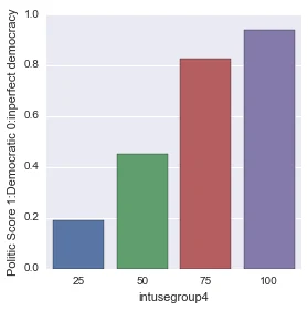
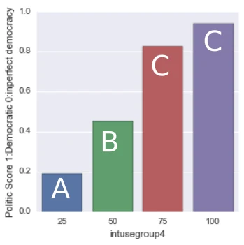
**Model Interpretation for Chi-Square Tests: **
When examining the association between Internet Use Rate (categorical response.. Grouped in 4 groups.0-25, 25-50, 50-75, 75-100) and Polity Score (categorical explanatory… Grouped in 1: Democratic Country and 0:Inperfect democracy ) a chi-square test of independence revealed that Internet Use Rate, those with more Internet Use Rate have is more apximate to a real democracy X2=49.069261660631597, P=1.2609118937138063e-10.
Model Interpretation for post hoc Chi-Square Test results:
A Chi Square test of independence revealed that Internet User Rate, And Polity Score. (binary categorical variable) were significantly associated, X2=49.069261660631597, P=1.2609118937138063e-10.
Post hoc comparisons of rates of Internet User Rate by pairs of categories revealed that higher rates of Polity Score. were seen among those Internet User Rate up to 50 to 100. In comparison, prevalence of Polity Score. was statistically similar among those groups smoking